For this project, I worked with a fake movie dataset to build a model predicting whether a film would be a success or a flop. The purpose of this project was to learn more about what data science entails and get a more general understanding of exploratory data analysis (EDA) and building models.
In this post, I'm going to walk you through the EDA (Univariate Graphical EDA to be specific) process and how I built this binary classification model. And I would like to strongly emphasize, this is my first time doing all this lol
Data Cleaning
After understanding the problem and inspecting the data, I moved on to cleaning the data. The data set had the following issues and here's how I resolved them:
- Incorrect scaling in budget data: Certain budgets were listed fully and not by millions. I applied a function to ensure all units were in millions.
def scale_to_million(num):
    if len(str(num).split(".")[0]) > 3:
        return num / 1000000
    return num

df['Budget'] = df['Budget'].apply(scale_to_million)- Outlier movie runtime values: Some movies had runtimes of 0 minutes and one value was a string instead of an integer. I imputed these values with the median runtime and dropped the non-integer value.
df['Runtime'] = pd.to_numeric(df['Runtime'], errors='coerce')
runtime_median = df[df['Runtime'] != 0]['Runtime'].median()
df['Runtime'].replace(0, runtime_median, inplace=True)
df['Runtime'].fillna(runtime_median, inplace=True)- Outlier star metrics: Two movies had 100 as their star rating, which is not realistic. I dropped these values as they represented only 0.37% of the data.
df = df[df['Stars'] < 6]Data Exploration
After cleaning the data, the next step in the EDA process is to "explore the data", i.e. pretty much just find trends. I broke down my exploration process into a couple questions:
Do seasons have a statistically significant impact on success?
I answered this question by running a chi-squared test on movie season and success.
contingency = pd.crosstab(df['Season'], df['Success'])
chi2, p_value, dof, expected = stats.chi2_contingency(contingency)
Answer: Yes (p-value = 0.0065... < 0.05)
Do seasons have a statistically significant distribution of ratings?
Like the question above, I answered this question by running a chi-squared test on movie season and ratings.
contingency = pd.crosstab(df['Season'], df['Rating'])
chi2, p_value, dof, expected = stats.chi2_contingency(contingency)
Answer: No (p-value = 0.2096... < 0.05)
Who is the harshest critic (highest percentage of negative reviews)?
To determine who the meanest critic was, I analyzed every review and assigned it a sentiment score. I used the Natural Language Toolkit for sentiment analysis.
from nltk.sentiment import SentimentIntensityAnalyzer
import nltk
nltk.download('vader_lexicon')

sia = SentimentIntensityAnalyzer()

def classify_sentiment(text):
    score = sia.polarity_scores(text)["compound"]
    return 'positive' if score > 0 else 'negative'

for column in ['R1', 'R2', 'R3']:
    df[column + ' sentiment'] = df[column].apply(classify_sentiment)

R1_percentage = df['R1 sentiment'].value_counts().get('negative', 0) / df['R1 sentiment'].count()
R2_percentage = df['R2 sentiment'].value_counts().get('negative', 0) / df['R2 sentiment'].count()
R3_percentage = df['R3 sentiment'].value_counts().get('negative', 0) / df['R3 sentiment'].count()

print(R1_percentage, R2_percentage, R3_percentage)
Turned out that R1 was the harshest critic (78.25% negative reviews).
What is the covariance between the promotional and filming budget?
Lastly, I found the covariance between promotional and filming budget.
covariance = df[['Budget', 'Promo']].cov().iloc[0, 1]The covariance was 1908.7277, which indicates a positive linear relationship between the two variables.
Data Visualization
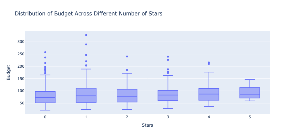
Next, I plotted some metrics to further evaluate the nature of the data. For example, I plotted the distribution of budget across the different number of stars to better guage the variety of budgets for each star and how the median budgets for each star compare to one another. Here's the plot:

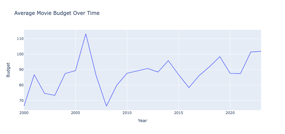
In the plot, we can see that the medians of every movie regardless of star remained between 50 to 100 million dollars. It also shows how there's less variation in movies with 4 and 5 stars compared to movies with 0 and 1 star. I also plotted the average movie budget over time shown below:

From 2000 to 2023, movie budgets generally grew over time pointed out by the positive trend in the graph with a spike around 2007. This is a good time to point out again that all of this data is fake and for practice.
Feature Engineering
After exploring trends and visualizing important attributes of the data, it was time to begin cooking up the classification model. To do this, I first began feature engineering to improve the model's performance by emphasizing signficant attributes and involving categorical effects. Here's what I added:
- Sentiment Scores Encoding (1 for positive, 0 for negative)
def assign_sentiment(sentiment):
    return 1 if sentiment == 'positive' else 0

df['R1 sentiment'] = df['R1 sentiment'].apply(assign_sentiment)
df['R2 sentiment'] = df['R2 sentiment'].apply(assign_sentiment)
df['R3 sentiment'] = df['R3 sentiment'].apply(assign_sentiment)- Season One-Hot Encoding
series = pd.Series(df['Season'])
one_hot = pd.get_dummies(series)
df = df.join(one_hot)
df.head()- Rating One-Hot Encoding
series = pd.Series(df['Rating'])
one_hot = pd.get_dummies(series)
df = df.join(one_hot)
df.head()- Genre One-Hot Encoding
series = pd.Series(df['Genre'])
one_hot = pd.get_dummies(series)
df = df.join(one_hot)
df.head()
Now with these encodings, I could factor in more attributes to my model by converting qualitative features to quantitative traits. This was important because each of the four chosen categories can have a significant impact on a movie.
Modeling
I chose an XGBoost Classifier because it uses an ensemble learning method based on gradient boosting, combining the predictions of several base decision trees. This helps in capturing different patterns and relationships in the data. Furthermore, XGBoost provides insights into feature importance, which is an important part of evaluating your model (we'll see this later). To balance the dataset, I downsampled the majority class and built the model accordingly:
from sklearn.utils import resample
from xgboost import XGBClassifier

df_majority = df[df.Success == False]
df_minority = df[df.Success == True]

# Downsample the majority class
df_majority_downsampled = resample(df_majority, replace=False, n_samples=len(df_minority), random_state=42)

df_balanced = pd.concat([df_majority_downsampled, df_minority])

X = df_balanced[['Runtime', 'Stars', 'Year', 'Budget', 'Promo', 'R1 sentiment', 'R2 sentiment', 'R3 sentiment', 'Fall', 'Spring', 'Summer', 'Winter', 'PG', 'PG13', 'R', 'Action', 'Drama', 'Fantasy', 'Romantic Comedy', 'Science fiction']]
y = df_balanced['Success']

xgb = XGBClassifier()
Testing
To test the model, I shuffled the data and split it into a 10% test set and 90% training set which is known as 10-fold cross validation.
from sklearn.model_selection import train_test_split
from sklearn.metrics import accuracy_score

X_train, X_test, y_train, y_test = train_test_split(X, y, test_size=0.1, random_state=0, shuffle=True)
xgb.fit(X_train, y_train)
y_pred = xgb.predict(X_test)
accuracy = accuracy_score(y_test, y_pred)
The testing provided us with a model accuracy of 79.1662%. Now initially, I would think to stop here once you obtain the model's accuracy. Data scientists, however, often prioritize other metrics as well such as false positive rate and false negative rate. We can obtain these values from what's called a confusion matrix.
from sklearn.metrics import confusion_matrix

cm = confusion_matrix(y_test, y_pred)
false_neg_rate = cm[1][0] / (cm[1][0] + cm[1][1])
false_pos_rate = cm[0][1] / (cm[0][0] + cm[0][1])
From the confusion matrix, I found the false negative rate to be 21.4286% and the false positive rate to be 20%. After evaluating all these metrics to gain a better understanding of how good our model is, I wanted to determine what the most important feature was.
xgb.get_booster().get_score(importance_type='total_gain')Turns out the most important feature was Budget. The importance type, total gain, refers to the amount of added information the budget feature provided the model with when making correct decisions.
Conclusion
This project gave me an in-depth introduction to data science by taking me through the procedures of data cleaning, exploration, visualization, feature engineering, and creating models. Working with a fictional movie dataset taught me how to deal with various data challenges, including inaccurate scaling, outliers, and missing data. The exploratory data analysis (EDA) helped me explore the connections across multiple features and their effects on film success.
An XGBoost classifier seemed to be a reasonable choice for this binary classification challenge since it is designed to handle structured data and provide insights into feature importance. The model had a decent accuracy of 79.1662%, with acceptable false positive and false negative rates.
Overall, this project was a great intro to data science and ML modeling. The primary takeaway was the significance of thorough data preprocessing and feature engineering in constructing beneficial machine-learning models. Furthermore, I grew more knowledgeable about the importance of evaluating metrics beyond just accuracy.
My background is primarily in software engineering, so going beyond implementing an open-source model and instead implementing my own was a great learning experience. In the future, I plan on reading more about how ML models are implemented at scale using tools such as Apache Spark and gaining a better understanding of MLOps in general.